Eurovision with Fabric: Part 2

This is part of a mini series on analysing Eurovision data with Microsoft Fabric. If you missed part one you can read it here. In part 1 I briefly covered the initial data load via the Youtube API and web scraping. So now we need to enhance this data to be ready for final analysis.

Mapping videos to countries

In the initial load of the videos table, the title for the video was returned by the API. However, in order to do meaningful analysis later we need to extract the country of the video. After a few attempts at working out a dynamic way to do this, such as going of flag emojis. However, due to the wide range of variations of title I eventually settled on just having a list of regex with one value for each country that has competed in Eurovision.

_{Regex Sample}

(r"(?i).*\bGreece\b.*", "Greece"),
(r"(?i).*\bHungary\b.*", "Hungary"),
(r"(?i).*\bIceland\b.*", "Iceland"),
(r"(?i).*\bIreland\b.*", "Ireland"),
(r"(?i).*\bIsrael\b.*", "Israel"),

With this regex list defined I then looped through this for every video to find a matching pattern. This code won’t handle if multiple patterns are matched but luckily that wasn’t an issue. There were some challenges with the initial patterns that were used where shorter country names, like Greece or Russia, were matching on song titles. To resolve this I added the word boundary flags within the patterns which resolved this.

country_expr = None
# Loop through each condition and check if the title column values match that pattern
for pattern, country in conditions:
    condition = F.col(title_col).rlike(pattern)
    if country_expr is None:
        country_expr = F.when(condition, F.lit(country))
    else:
        country_expr = country_expr.when(condition, F.lit(country))

# Add handling for if no condition is met, set the country as Unknown.
country_expr = country_expr.otherwise(F.lit("Unknown"))

return df.withColumn("country", country_expr)

Creating an overall rank

The next data enhancement is to the results data that was scraped from Wikipedia. The data as is doesn’t have an overall result for each competition, only a placement within the final and semi finals. This means we can’t compare across years if a country didn’t make the final for every year we are looking at. This is also further complicated as the number of countries participating changes year to year. To solve all this the plan was to create a ranking with the finals used first and then points within a semi final for countries that didn’t qualify to the final.

As the data returned from the beautiful soup web scraping is based on raw HTML it is quite messy with notes and non numeric values. First we need to remove the notes which are square brackets containing references/notes such as additional context within the wikipedia page.

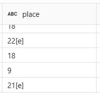
In order to remove these we can use regex to remove the square brackets and any text within.

columns_to_clean = ["country", "artist", "song", "place", "sf_place", "points", "sf_points"]
for column in columns_to_clean:
    results_df = results_df.withColumn(column,F.trim(F.regexp_replace(F.col(column), r"\[.*?\]", "")))

Once this is done the only remaining issue left to clean is replacing “-” characters with null so the data can be cast to a number.

results_df = results_df \
    .withColumn("place", F.when(F.col("place") == "—", None).otherwise(F.col("place"))) \
    .withColumn("points", F.when(F.col("points") == "—", None).otherwise(F.col("points")))

Now the data is clean we can start enhancing it for later analysis. The first of these steps is adding a rank for each year across the semi final and final of each year. First we need to find how many countries were in the final, which we can calculate from the maximum place within each year. Then for countries that did not make the final we rank them by the amount of points they got in the semi final. Both of these are done with two simple windows.

# Define a window partitioned by year to compute maximum final placement ("place").
year_window = Window.partitionBy("year")

# Define a window over rows (per year) ordering by sf_points descending.
window_spec = Window.partitionBy("year").orderBy(F.col("sf_points").desc())

# Create the new "new_place" column:
# - When "place" is non-null, use it directly.
# - Otherwise, compute new_place as: COALESCE(max(place) over year, 0) + row_number over the rank_window.
results_df = results_df.withColumn("max_final", F.max(F.col("place")).over(year_window)).withColumn("row_num", F.row_number().over(window_spec)) \
    .withColumn(
        "non_null_count", 
        F.coalesce(
            F.sum(F.when(F.col("place").isNotNull(), F.lit(1))).over(window_spec.rowsBetween(Window.unboundedPreceding, -1)),
            F.lit(0)
        )
    ) \
    .withColumn(
        "all_rank", 
        F.when(
            F.col("place").isNull(), 
            F.col("max_final") + F.col("row_num") - F.col("non_null_count")
        ).otherwise(F.col("place")).cast(T.IntegerType())
    )\
    .drop("max_final","row_num","non_null_count")

The final task to enable the analysis on results is joining on the video id based on the country and year so in future we can link the how popular the video is with the actual performance in the contest.

videos_with_year = videos_with_year.dropDuplicates(["vid_year","vid_country"])
output_df = results_df\
    .join(videos_with_year, [results_df.year == videos_with_year.vid_year,results_df.country == videos_with_year.vid_country], "left_outer")\
    .select(
        "year",
        "country",
        "artist",
        "song",
        "video_id",
        "place",
        "points",
        "semi_final",
        "sf_points",
        "sf_place",
        "all_rank",
        "_created_date",
        "_modified_date"
    )\
    .withColumn("video_id", F.coalesce(F.col("video_id"), F.lit("Unknown")))

SynapseML: Language classification & sentiment analysis

The final enhancement is to perform sentiment analysis on the video comments. For this Fabric has a set of built in AI functions in the SynapseML library. However, before performing sentiment analysis we first have to filter the comments down to supported languages, helpfully there is also a SynapseML function for language detection.

With this we can detect the language of each comment.

model = (AnalyzeText()
        .setTextCol("textDisplay")
        .setKind("LanguageDetection")
        .setOutputCol("response")
)

comments_with_lang = model.transform(raw_comments)\
        .withColumn("detectedLanguage", F.col("response.documents.detectedLanguage.name"))\
        .withColumn("detectedLanguageIso", F.col("response.documents.detectedLanguage.iso6391Name"))

Then from there we can filter down to the ones supported for sentiment analysis.

supported_languages = {'af',...,'yi'}
comments_supported = comments_with_lang.where(F.col('detectedLanguageIso').isin(supported_languages))

With the supported comments, the sentiment can be detected.

model = (AnalyzeText()
        .setTextCol("textDisplay")
        .setKind("SentimentAnalysis")
        .setOutputCol("response")
)

comments_with_sentiment = model.transform(new_or_modified_comments)\
        .withColumn("sentiment", F.col("response.documents.sentiment"))\
        .withColumn("positiveConfidence", F.col("response.documents.confidenceScores.positive"))\
        .withColumn("neutralConfidence", F.col("response.documents.confidenceScores.neutral"))\
        .withColumn("negativeConfidence", F.col("response.documents.confidenceScores.negative")
)

One final transformation of note is I added a hash column for the comment, this helps with merging in changes by making the comparisons on the hash rather than the full comment string.

A word of warning

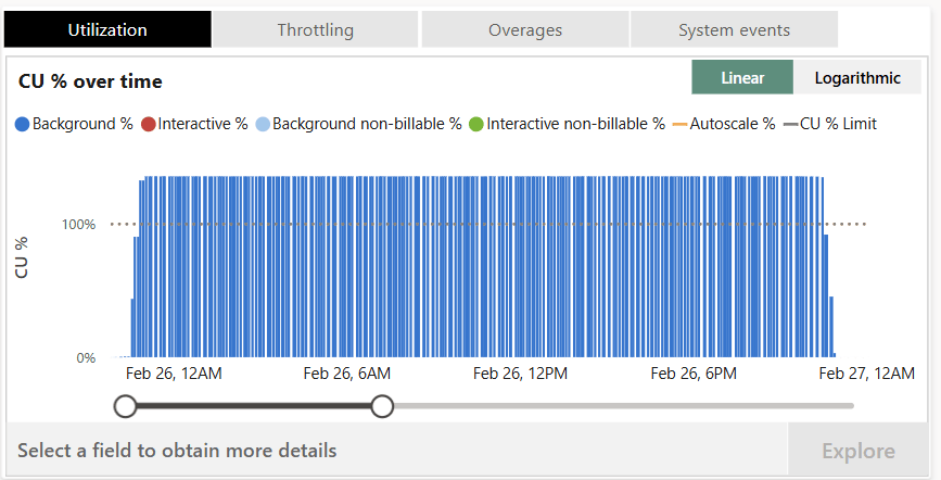
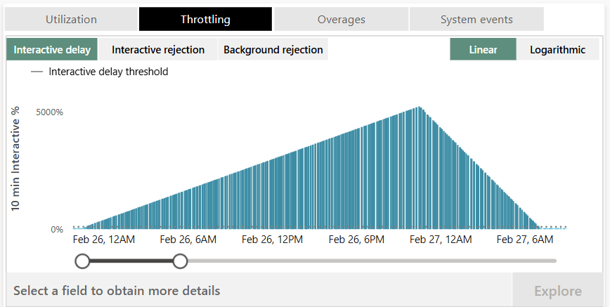
The SynapseML libraries can use a LOT of your capacities compute. The first time I ran the sentiment analysis the notebook used so many CUs that the background job used around 120% of a trial F64 capacity for a full day. This constant overload build up so much that it add interactive delay for over 36 hours! So make sure to test on a small data sample size then see how much that would scale to your full dataset. Otherwise you might effectively disable your entire capacity for multiple days!

If you do run into significant throttling and you aren’t on a trial capacity you can restore it to a useable state by scaling or pausing your capacity.

_{Capacity overload}

_{Capacity throttling}

Next part

You can read the next part of this mini series here.

• Fabric
• Power-Bi
• Data-Engineering